Aero: Virtual Cycling Wind Tunnel - Technical Breakdown

Blake Sanie | Feb 1, 2024

Progressing along my endurance triathlon adventure during the cold winter means crafting an indoor training regiment without compromise. Yes, I converted my bike into a stationary rig and sprinted away on virtual routes (all standard practice), though diving deeper, I sought a way to optimize my body positioning before hitting the road again in the spring.

My search for existing tools turned empty - applying advanced kinematic theory within a computationally defined environment seemed too much of a moonshot, especially when targetting a consumer hardware runtime. Still, no reason stood to prove my vision unattainable.

Being equal parts athletic competitor and technological innovator, I took matters into my own hands.

Creating Aero

To kick off 2024, I designed and developed Aero - the world’s first consumer-accessible virtual wind tunnel, focused on helping cyclists minimize air resistance due to suboptimal body geometry. Even better, complete functionality sits right behind the same web browser you are using to read this.

Finding success in Aero’s creation required seamlessly stitching together advanced applications of physical mechanics and machine learning. The below sections outline and further dissect these respective components.

Physics Theory, Applied

Rocketing at significant speeds through the still air simplifies to the disruption of a fluid at equilibrium. In the most basic of forms, air resistance increases linearly with respect to cross-sectional area, and quadratically with respect to velocity:

$F_{D}=\frac{1}{2}\rho v^2 C_D A$

with drag force $F_D$ , fluid density $\rho$ , velocity $v$ , drag coefficient $C_D$ , and cross sectional area $A$ . However, this baseline kinematic model relies on many material generalizations and does not consider chaotic fluid dynamics (i.e. turbulent flow) that result from nontrivial object shapes and positions. My desire to model the effects of arbitrary body shapes eliminate all possibilities of a closed-form approximation for air resistance. Putting pen and paper aside, pivoting towards a simulation-based approach allows for situational precision while leveraging academically studied numerical and computational methods.

Modelling Fluid Dynamics

Cutting-edge fluid simulation methods follow one of two paradigms.

Eulerian approaches discretize and fix the environment (grid or mesh), each managing fluid behavior within their respective bounds.
LaGrangian approaches discretize and fix the fluid (as particles), each managing their respective state (position, velocity, etc) within the environment.

Aero’s fluid simulation relies on an Eulerian method to ensure uniform measurement across the environment while easily parallelizing underlying grid-based computations.

Deeper, I evolved the Lattice-Boltzmann Algorithm to support the platform’s wind tunnel dynamics - more on improvements later. The method operates as follows:

Form a lattice-structured environment, where each cell of the environment grid stores an eight-way particle distribution: moving North, North-East, East, South-East, South, South-West, West, North-West, and staying at rest. The density of particles in each category are initialized to reflect a constant rate of laminar flow (a state of equilibrium that observes the Navier-Stokes Equations).
Propogate the expected densities to the corresponding cell. For instance, transfer the density of North-traveling particles to the cell above the current. Careful formulation of this sequential process is necessary to ensure densities are not overwritten while still a dependency in pending computations. This is called the “Stream” step. Handle collisions by reflecting movement into barriers back onto the source cell.
Smooth each cell’s new fluid movement distribution towards an equilibrium state. This “Collide” phase introduces nonlinearity to fluid movement - a realistic mechanism to handle movement dampening and compounding. Find an in-depth explanation of the relevant mathematical foundation here.
Jump to step 2, forming a cycle that models the passage of time.

A few details in technical implementation require attention to complete an effective simulation. These include:

Resetting environment boundaries to uniform equilibrium density (repeat as step 1 at edges of the canvas) to keep the fluid moving in the intended direction. This can happen with any time interval, though tighter intervals promote simulation stability.
Dynamically shifting the initial air flow point (front of the wind tunnel) to accommodate the object’s shape and position within the wind tunnel. This extension to the Lattice-Boltzmann algorithm prevents differences in fluid behavior across ends of the wind tunnel because the object’s position relative within the wind tunnel is unchanging.

Relating Speed, Position, Power, and Force

With the appropriate simulation method by my side, I then needed a quantitative model between the measures of interest. As a starting point, I discovered the below real-world data aggregated by the team at Silca relates power savings and cycling speed in various body positions.

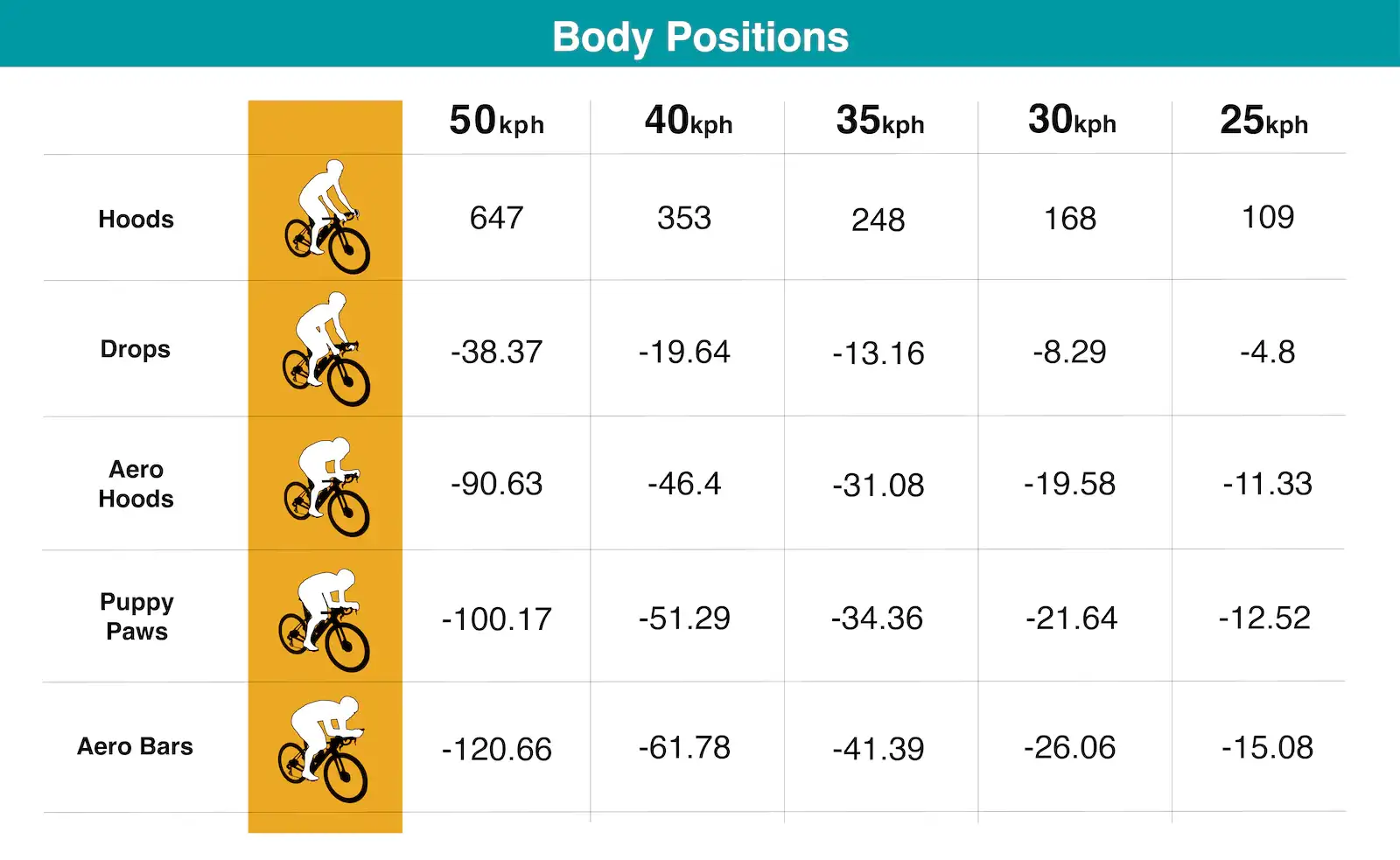
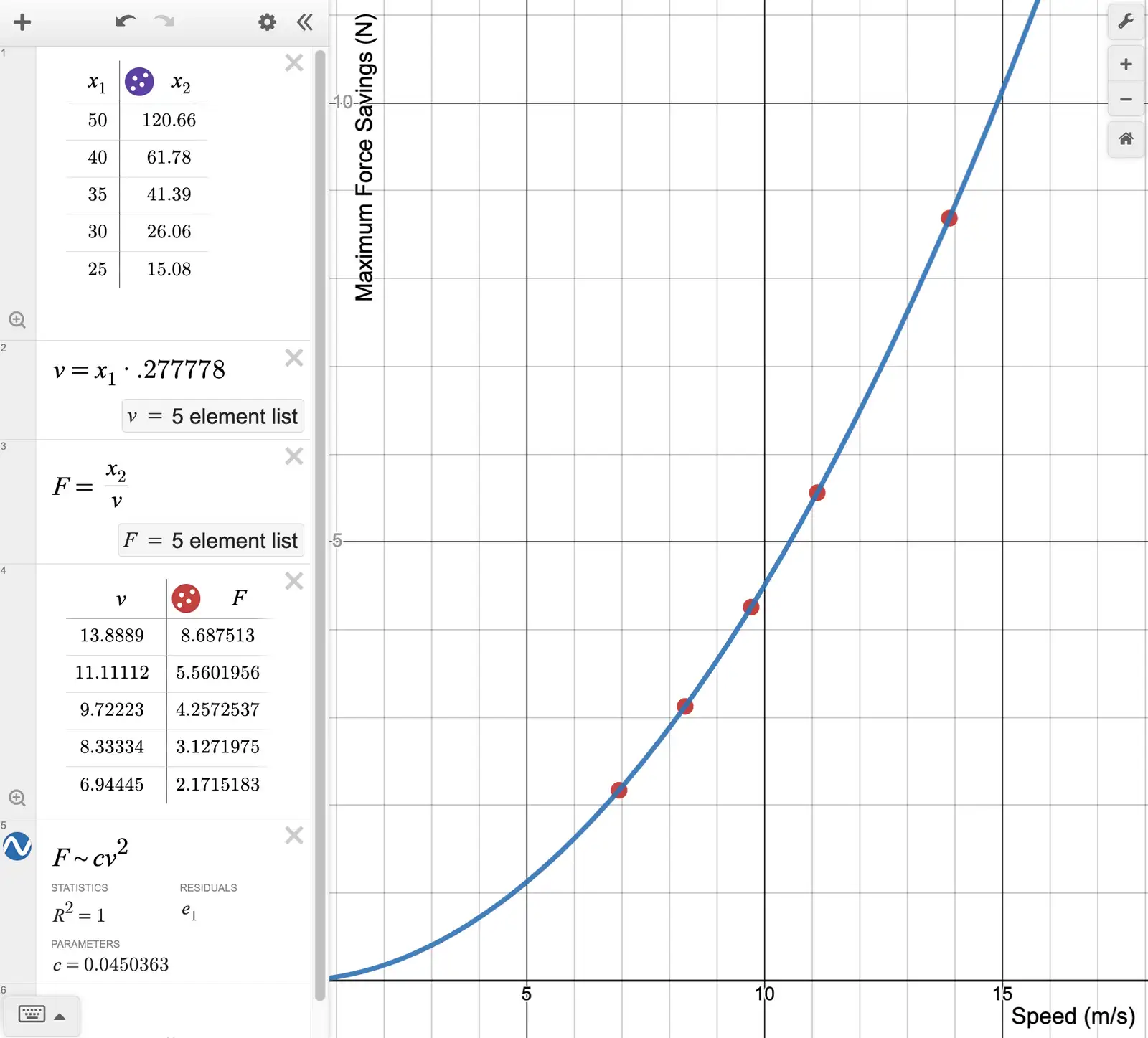
Power savings with body positions versus speed, by Silca.

I am mainly interested in modeling maximum power savings, which occurs in the Aero Bars position. Using this Desmos plot, I found the relationship between maximum force savings (N) and cycling speed (m/s) to be:

$F_\text{saved}=c v^2,\hspace{2mm} c=.0450363$

Which maintains the quadratic order held by the ideal drag force equation!

Regression model between cycling speed and maximum force savings.

At this point, I needed a means of relating simulation mechanics to the above regression model. The simulation progresses with a frame rate $f=24$ frames per second, with each frame running $n=40$ iterations of the “Streaming” and “Colliding” process.

During the computation of each frame, I accumulate the mass colliding in the net $x$ and $y$ directions across all barrier cells $B$ (areas occupied by the bike and cyclist). Together, these components form a vector $\vec{m_\text{air}}$ .

$m_{\text{air}_x}=\sum_{i=0}^{n}\sum_{b\in B}(\text{NE}_b + \text{E}_b + \text{SE}_b - \text{SW}_b - \text{W}_b - \text{NW}_b)$

$m_{\text{air}_y}=\sum_{i=0}^{n}\sum_{b\in B}(\text{SW}_b + \text{S}_b + \text{SE}_b - \text{NE}_b - \text{N}_b - \text{NW}_b)$

$\vec{m_\text{air}}=\langle m_{\text{air}_x},m_{\text{air}_y} \rangle$

On the road, the cyclist’s kinetic energy is lost to the surrounding air. Analogously, the air in the wind tunnel transfers its kinetic energy into the body. The amount of work (joules), or change in energy, subjected to the body is expressed as:

$\vec{W_\text{air}} = \frac{1}{2}\vec{m_\text{air}}v^2$

Further, the air resistance force vector is found by applying the computed work over the traversed distance, which is itself the quotient of velocity and frame rate.

$\vec{F_\text{air}} = \vec{W_\text{air}} \Delta x,\hspace{2mm}\Delta x = v \Delta t = \frac{v}{f}$

Keep in mind that a cyclist must combat a horizontal force working against them, however, $\vec{F_\text{air}}$ has an unconsidered vertical component. This detail should not be overlooked, as $F_{\text{air}_y}$ induces an increase in Rolling Resistance, $F_\text{rr}$ , which is a horizontally acting force on the cyclist. $C_\text{rr}=0.004$ is the empirical rolling resistance constant for road tires with intended pressure on smooth asphault, found by Silca.

$F_\text{resistance} = F_{\text{air}_x} + F_\text{rr}$

$F_\text{rr} = C_\text{rr} F_{\text{air}_y},\hspace{2mm} C_\text{rr} = 0.004$

Chasing Power and Force Savings

At this point, relative values of $F_\text{resistance}$ hold physically accurate, but the values in absolute may be inflated by barrier configuration, simulation speed, and scene width, among other external variables. I eliminate the effect of these factors by imposing a calibration step - for 10 seconds, the cyclist alternates between a “Hoods” position to record $\dot{F}_\text {high}$ (baseline for zero force savings) and the lowest possible “Aero Bars” position to record $\dot{F}_\text{low}$ (baseline for maximum force savings). Here, all forces vary in third degree with speed, tracing all derivations steps. Thus, $\dot {F}_\text {high}$ and $\dot{F}_\text{low}$ take into account a $v^3$ normalization factor so that the baselines remain valid independent of airspeed, which may change throughout the simulation. To recompute force from the baseline space, a factor of $v^3$ is applied. Once calibrated, force savings are quickly estimated by interpolating the normalized observed horizontal resistance force between the two bounds and scaling the force savings regression model accordingly.

$F_\text{saved} = v^3 * \frac{\dot{F}_\text{high} - F_\text{resistance}/ v^3}{\dot{F}_\text{high}-\dot{F}_\text{low}} * cv^2$ $= \frac{\dot{F}_\text{high} - F_\text{resistance}/ v^3}{\dot{F}_\text{high}-\dot{F}_\text{low}} cv^5$ $P_\text{saved} = F_\text{saved}v$

Computer Vision Considerations

The proposed theoretical physics backing only holds half the weight of the simulation - missing is environment formulation and interactivity. To achieve this, I rely on a key computer vision method: Image Segmentation.

Image Segmentation

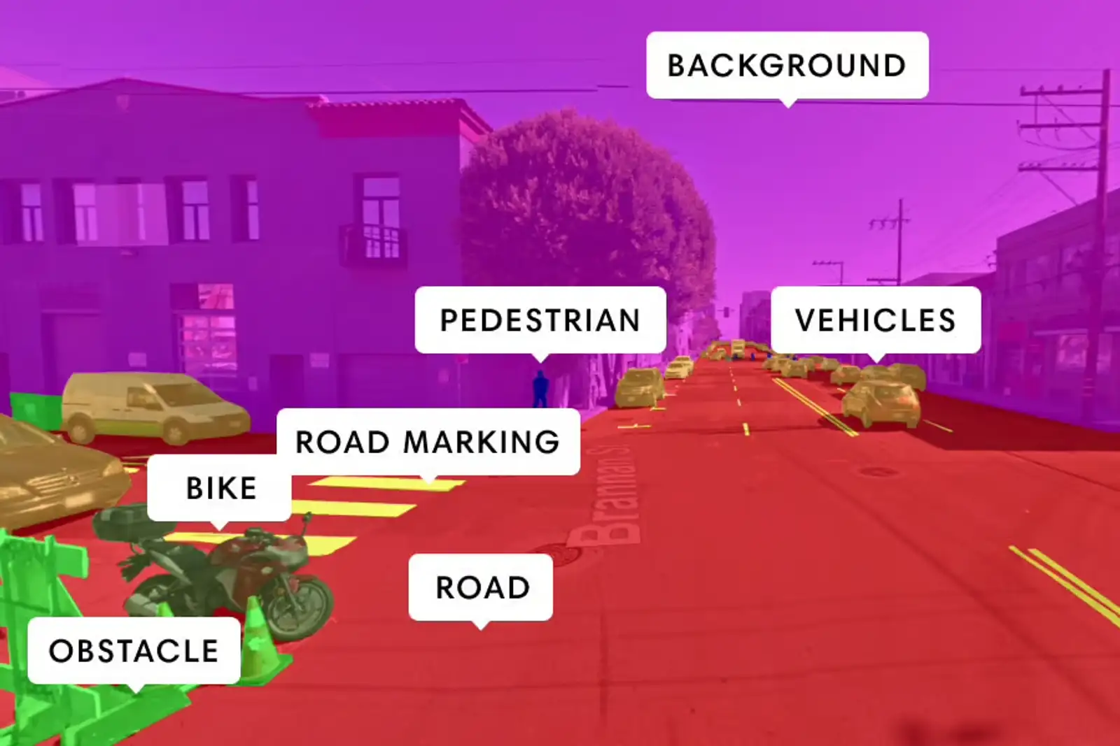
To enable detection of the cycle and cyclist in real time using only the device’s webcam, I leverage a machine learning-based method called semantic image segmentation. In short, a segmentation model takes an image as input and analyzes its features to extract visual information from within. The output, microscopically, embodies a pixel-wise classification result. Is this pixel belonging to a cycle or cyclist, or something else? These values are represented probabilistically. Macroscopically, these pixel classifications join to assign image regions to object categories. This is the same computer vision technology that drives cutting-edge autonomous vehicle perception, picture below.

Semantic image segmentation output example by scale.com (Scale AI).

Barrier Detection Workflow

With this model up and running, we may capture stills from the video webcam feed and invoke inference. Once the output is collected, it is converted into a boolean mask, where true represents a barrier (dominant cycle or cyclist classification), or false otherwise. This mask is then resized to fit the dimensions of the discretized simulation algorithm and subsequently rendered onscreen. Because running a machine learning model in continuation requires high computational cost, other app processes such as the simulation itself may see less priority by the page’s process scheduler. Hence, choosing a segmentation inference interval that balances smooth, real-time updates with a reasonable computation budget. This task is also aided by improving computational efficiency across this process itself. Let’s dive deeper.

Web-Optimized Implementation and Runtime

Today, it is fairly uncommon to have high-intensity machine learning models run client-side in the browser. The main reason for this is excess computation time and resource overload, as mentioned, which can be avoided by invoking the machine learning task on the backend. This design pattern works effectively for one-time tasks with low data volume, such as a basic chat. However, continuously streaming video or image data to a backend invites a new computational bottleneck to the party - network I/O. Therefore, if the model is suitably compact, it is more appropriate to load the model once over the network, and then dispatch inference tasks locally as needed.

One of the primary industry-standard frameworks for machine learning development is Google’s Tensorflow. The toolkit’s greatest strengths lie in its Python package, which is central to model training, experimentation, and export. Deployment and real-world model usage present a few more options, one of which is the web-enabling Tensorflow.js runtime.

The high-level workflow is simple - load the framework with the webpage, pull down the model of choice, and perform inference by casting to/from Tensorflow.js compatible datatypes.

Model Optimization and Memory Management

Effective and robust models are not slim. My model of choice has over 50 million fine-tuned parameters to support its intelligent process. Quantization is a method to reduce model size without sacrificing parameter count. Model parameters are typically stored as 32-bit floats: high precision with high payload. Such parameters may be quantized to a smaller representation, settling for less-than-perfect precision to fit an 8 or 16-bit representation.

I opted for 8-bit quantization to fully minimize model loading time (streaming fewer bytes over the network) and simultaneously minimize memory footprint within the page’s browser process. In the end, this precision sacrifice is hardly felt, since the dominant pixel-wise classifications remain accurate and each region retrains a refined boundary.

Tensorflow.js also allows for programmatic memory management. Although its tensor datatypes occupy large heaps of memory, we can free these blocks as soon as they become obsolete. Utilization of this feature is especially critical when considering that all operations return a new tensor - pipelining a series of operations creates many auxiliary tensor objects, none of which are needed except the final output. Purging unused tensors as the inference step progresses keeps memory usage as tidy as possible, thus keeping machine learning in the browser as feasible as possible.

Hardware Optimization for Machine Learning

Further, Tensorflow.js builds upon tensor computation, where data is stored contiguously in memory for fast access and efficient computation. These operations consist of matrix calculations commonly found in computer graphics processing. Along this connection is the Web Graphics Library (WebGL), a high-performance graphics engine with near-ubiquitous browser compatibility. Though designed for direct rending tasks, its underlying matrix operation capability allows for machine learning tensor computation to live closer to accelerated hardware, such as GPUs. This technology closes the gap between standard JavaScript execution in the browser and the unbounded local computation ability of Tensorflow’s Python framework.

Tensorflow.js is smart enough to detect WebGL compatibility with your browser, leveraging the underlying hardware acceleration if possible, and defaulting to standard JavaScript computation otherwise. As a result, all browsers support the model’s execution, with all hardware-driven performance gains applied where possible.

Closing Thoughts

The vision behind Aero came to life thanks to numerous key mathematical and computational modeling considerations, not to mention an optimization-focused technical execution within the runtime constraints of a web browser. Scratch paper, debuggers, and head-banging of the past aside, go save some Watts!